
Seaborn Styling, Part 1: Figure Style and Scale
Seaborn Styling, Part 1: Figure Style and Scale
Introduction
When creating a data visualization, your goal is to communicate the insights found in the data. While visualizing communicates important information, styling will influence how your audience understands what you’re trying to convey.
After you have formatted and visualized your data, the third and last step of data visualization is styling. Styling is the process of customizing the overall look of your visualization, or figure. Making intentional decisions about the details of the visualization will increase their impact and set your work apart.
In this article, we’ll look at how to do the following techniques in Seaborn:
- customize the overall look of your figure, using background colors, grids, spines, and ticks
- scale plots for different contexts, such as presentations and reports
Customizing the Overall Look of Your Figure
Seaborn enables you to change the presentation of your figures by changing the style of elements like the background color, grids, and spines. When deciding how to style your figures, you should take into consideration your audience and the context. Is your visualization part of a report and needs to convey specific information? Or is it part of a presentation? Or is your visualization meant as its own stand-alone, with no narrator in front of it, and no other visualizations to compare it to?
In this section, we’ll explore three main aspects of customizing figures in Seaborn - background color, grids, and spines - and how these elements can change the look and meaning of your visualizations.
Built-in Themes
Seaborn has five built-in themes to style its plots:darkgrid,whitegrid,dark,white, andticks. Seaborn defaults to using thedarkgridtheme for its plots, but you can change this styling to better suit your presentation needs.
To use any of the preset themes pass the name of it tosns.set_style().
sns.set_style("darkgrid")sns.stripplot(x="day", y="total_bill", data=tips)
Copy to clipboard
sns.set_style("darkgrid")sns.stripplot(x="day", y="total_bill", data=tips)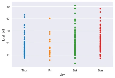
image1
We’ll explore the rest of the themes in the examples below.
Background Color
When thinking about the look of your visualization, one thing to consider is the background color of your plot. The higher the contrast between the color palette of your plot and your figure background, the more legible your data visualization will be. Fun fact: dark blue on white is actually more legible than black on white!
Thedarkbackground themes provide a nice change from the Matplotlib styling norms, but doesn’t have as much contrast:
sns.set_style("dark")sns.stripplot(x="day", y="total_bill", data=tips)
Copy to clipboard
sns.set_style("dark")sns.stripplot(x="day", y="total_bill", data=tips)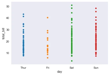
image2
Thewhiteandtickthemes will allow the colors of your dataset to show more visibly and provides higher contrast so your plots are more legible:
sns.set_style("ticks")sns.stripplot(x="day", y="total_bill", data=tips)
Copy to clipboard
sns.set_style("ticks")sns.stripplot(x="day", y="total_bill", data=tips)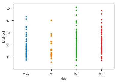
image3
Grids
In addition to being able to define the background color of your figure, you can also choose whether or not to include a grid. Remember that the default theme includes a grid.
It’s a good choice to use a grid when you want your audience to be able to draw their own conclusions about data. A grid allows the audience to read your chart and get specific information about certain values. Research papers and reports are a good example of when you would want to include a grid.
sns.set_style("whitegrid")sns.stripplot(x="day", y="total_bill", data=tips)
Copy to clipboard
sns.set_style("whitegrid")sns.stripplot(x="day", y="total_bill", data=tips)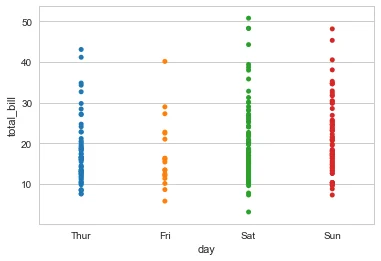
image4
There are also instances where it would make more sense to not use a grid. If you’re delivering a presentation, simplifying your charts in order to draw attention to the important visual details may mean taking out the grid. If you’re interested in making more specific design choices, then leaving out the grids might be part of that aesthetic decision.
sns.set_style("white")sns.stripplot(x="day", y="total_bill", data=tips)
Copy to clipboard
sns.set_style("white")sns.stripplot(x="day", y="total_bill", data=tips)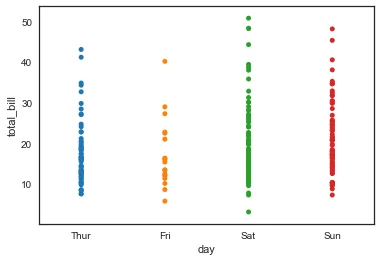
image5
In this case, a blank background would allow your plot to shine.
Despine
In addition to changing the color background, you can also define the usage ofspines. Spines are the borders of the figure that contain the visualization. By default, an image has four spines.
You may want to remove some or all of the spines for various reasons. A figure with the left and bottom spines resembles traditional graphs. You can automatically take away the top and right spines using thesns.despine()function. Note: this function must be called after you have called your plot.
sns.set_style("white")sns.stripplot(x="day", y="total_bill", data=tips)sns.despine()
Copy to clipboard
sns.set_style("white")sns.stripplot(x="day", y="total_bill", data=tips)sns.despine()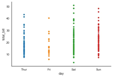
image6
Not including any spines at all may be an aesthetic decision. You can also specify how many spines you want to include by callingdespine()and passing in the spines you want to get rid of, such as: left, bottom, top, right.
sns.set_style("whitegrid")sns.stripplot(x="day", y="total_bill", data=tips)sns.despine(left=True, bottom=True)
Copy to clipboard
sns.set_style("whitegrid")sns.stripplot(x="day", y="total_bill", data=tips)sns.despine(left=True, bottom=True)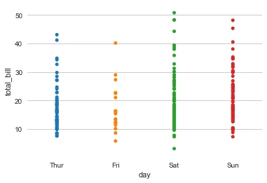
image7
Scaling Figure Styles for Different Mediums
Matplotlib allows you to generate powerful plots, but styling those plots for different presentation purposes is difficult. Seaborn makes it easy to produce the same plots in a variety of different visual formats so you can customize the presentation of your data for the appropriate context, whether it be a research paper or a conference poster.
You can set the visual format, or context, usingsns.set_context()
Within the usage ofsns.set_context(), there are three levels of complexity:
- Pass in one parameter that adjusts the scale of the plot
- Pass in two parameters - one for the scale and the other for the font size
- Pass in three parameters - including the previous two, as well as thercwith the style parameter that you want to override
Scaling Plots
Seaborn has four presets which set the size of the plot and allow you to customize your figure depending on how it will be presented.
In order of relative size they are:paper,notebook,talk, andposter. Thenotebookstyle is the default.
sns.set_style("ticks")    # Smallest context:sns.set_context("paper")sns.stripplot(x="day", y="total_bill", data=tips)
Copy to clipboard
sns.set_style("ticks") # Smallest context:sns.set_context("paper")sns.stripplot(x="day", y="total_bill", data=tips)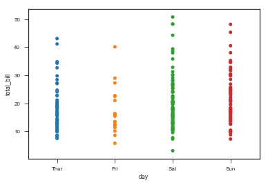
image8
sns.set_style("ticks")    # Largest Context:sns.set_context("poster")sns.stripplot(x="day", y="total_bill", data=tips)
Copy to clipboard
sns.set_style("ticks") # Largest Context:sns.set_context("poster")sns.stripplot(x="day", y="total_bill", data=tips)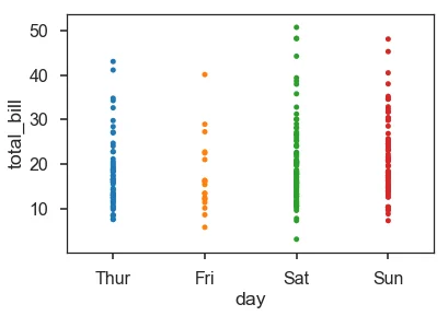
image9
Scaling Fonts and Line Widths
You are also able to change the size of the text using thefont_scaleparameter forsns.set_context()
You may want to also change the line width so it matches. We do this with thercparameter, which we’ll explain in detail below.
# Set font scale and reduce grid line width to matchsns.set_context("poster", font_scale = .5, rc={"grid.linewidth": 0.6})sns.stripplot(x="day", y="total_bill", data=tips)
Copy to clipboard
# Set font scale and reduce grid line width to matchsns.set_context("poster", font_scale = .5, rc={"grid.linewidth": 0.6})sns.stripplot(x="day", y="total_bill", data=tips)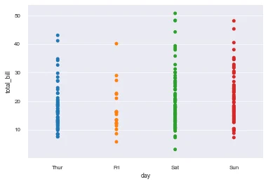
image10
While you’re able to change these parameters, you should keep in mind that it’s not always useful to make certain changes. Notice in this example that we’ve changed the line width, but because of it’s relative size to the plot, it distracts from the actual plotted data.
# Set font scale and increase grid line width to matchsns.set_context("poster", font_scale = 1, rc={"grid.linewidth": 5})sns.stripplot(x="day", y="total_bill", data=tips)
Copy to clipboard
# Set font scale and increase grid line width to matchsns.set_context("poster", font_scale = 1, rc={"grid.linewidth": 5})sns.stripplot(x="day", y="total_bill", data=tips)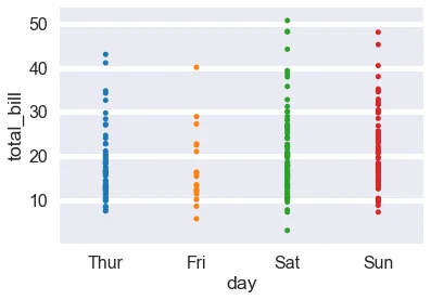
image11
The RC Parameter
As we mentioned above, if you want to override any of these standards, you can usesns.set_contextand pass in the parameterrcto target and reset the value of an individual parameter in a dictionary.rcstands for the phrase ‘run command’ - essentially, configurations which will execute when you run your code.
sns.set_style("ticks")sns.set_context("poster")sns.stripplot(x="day", y="total_bill", data=tips)sns.plotting_context()
Copy to clipboard
sns.set_style("ticks")sns.set_context("poster")sns.stripplot(x="day", y="total_bill", data=tips)sns.plotting_context()Returns:
{'axes.labelsize': 17.6, 'axes.titlesize': 19.200000000000003, 'font.size': 19.200000000000003, 'grid.linewidth': 1.6, 'legend.fontsize': 16.0, 'lines.linewidth': 2.8000000000000003, 'lines.markeredgewidth': 0.0, 'lines.markersize': 11.200000000000001, 'patch.linewidth': 0.48, 'xtick.labelsize': 16.0, 'xtick.major.pad': 11.200000000000001, 'xtick.major.width': 1.6, 'xtick.minor.width': 0.8, 'ytick.labelsize': 16.0, 'ytick.major.pad': 11.200000000000001, 'ytick.major.width': 1.6, 'ytick.minor.width': 0.8}
Copy to clipboard
{'axes.labelsize': 17.6, 'axes.titlesize': 19.200000000000003, 'font.size': 19.200000000000003, 'grid.linewidth': 1.6, 'legend.fontsize': 16.0, 'lines.linewidth': 2.8000000000000003, 'lines.markeredgewidth': 0.0, 'lines.markersize': 11.200000000000001, 'patch.linewidth': 0.48, 'xtick.labelsize': 16.0, 'xtick.major.pad': 11.200000000000001, 'xtick.major.width': 1.6, 'xtick.minor.width': 0.8, 'ytick.labelsize': 16.0, 'ytick.major.pad': 11.200000000000001, 'ytick.major.width': 1.6, 'ytick.minor.width': 0.8}Conclusion
As you can see, Seaborn offers a lot of opportunities to customize your plots and have them show a distinct style. The color of your background, background style such as lines and ticks, and the size of your font all play a role in improving legibility and aesthetics.
'The Codecademy Team, composed of experienced educators and tech experts, is dedicated to making tech skills accessible to all. We empower learners worldwide with expert-reviewed content that develops and enhances the technical skills needed to advance and succeed in their careers.'
Complete Payment to Unlock Full Guide & Source Code
You are viewing the 30% preview. Join TopCourseAI Pro to unlock the remaining 70% of this article, unblur all code snippets, and gain full access to all 412 technical projects and guides.
Ready to access the complete step-by-step tutorial?
Gain full unhindered access to all 412 technical projects and guides, unblur all source code snippets, and download runnable scripts.
Seaborn Color Palettes: Complete Guide to Data Visualization Colors
Next BlueprintSet Up with Git and GitHub
Related Blueprints & Guides
View all 166 →Creating a Word Cloud With Python
In Data Visualization,word cloudsare used to display textual data in a specific shape. The more frequent a word is in a chunk of text, the larger it will appear in the word cloud. This can provide interesting insights in...
Data visualizationData Visualizations for Messy Data
Data visualization tutorials generally use pre-processed data. But what about datasets in the wild? What do we do about missing data? Or outliers that largely skew visualizations? What do we do when there are too many ob...
Data visualizationEDA Prior To Fitting a Regression Model
Before fitting any model, it is often important to conduct an exploratory data analysis (EDA) in order to check assumptions, inspect the data for anomalies (such as missing, duplicated, or mis-coded data), and inform fea...
Ready to build production-grade AI systems?
Enjoyed this guide? Continue exploring our library of 166+ production blueprints, multi-agent swarms, and autonomous agent systems with 100% unblurred, executable source code.