
EDA Prior To Fitting a Regression Model
EDA Prior To Fitting a Regression Model
Introduction
Before fitting any model, it is often important to conduct an exploratory data analysis (EDA) in order to check assumptions, inspect the data for anomalies (such as missing, duplicated, or mis-coded data), and inform feature selection/transformation. In this article, we will usepandasto explore some of the EDA techniques that are generally employed prior to fitting a regression model.
The data
For our example analysis, we’ve downloaded a dataset fromKagglewhich contains data on Major League Baseball (MLB) games from the 2016 season. We’ve saved this data as aDataFramenamedbb. Suppose that we want to fit a linear regression to predictattendanceusing the following predictors:
- game_type— is the game during the day or at night?
- day_of_week— what day of the week did the game occur?
- temperature— average game temperature (Fahrenheit).
- sky— description of sky condition at the time of the game.
- total_runs— total runs scored in the game.
Preview the dataset
Any EDA process will probably begin by inspecting a subset of data. For apandasDataFrame, this can be done by using the.head()method:
bb.head()
Copy to clipboardbb.head()By looking at the first few rows of the data, we can often figure out what kind of data we have (eg., discrete or continuous) and get a sense of how they are coded. For example, we can see thatattendance,temperature, andtotal_runsare numbers, whilegame_type,day_of_week, andskyappear to be text.
After our initial inspection, we’ll want to dig deeper to investigate the following:
- The data type of each variable.
- How discrete/categorical data is coded (and whether we need to make any changes).
- How the data are scaled.
- Whether there is missing data and how it is coded.
- Whether there are outliers.
- The distributions of continuous features.
- The relationships between pairs of features.
Data types
It is important to check the data type for each feature. The quantitative variables should be read in as numbers — eitherint64orfloat64— and categorical variables should be stored as strings (columns ofstringshave adtypeofobjectbecause of how they are stored in Python). We can check data types of columns in a pandasDataFrameusing the.dtypesproperty.
bb.dtypes
Copy to clipboardbb.dtypesThe output will look like this:
attendance     float64
game_type       object
day_of_week     object
temperature     object
sky             object
total_runs      object
dtype: object
From this output, we can see thattemperatureandtotal_runsare both quantitative variables but they were read in asobjectdtypes. This can happen when there is a non-numeric character — such as a letter or punctuation symbol — in the same column. We would need to explore further in order to figure out what’s going on. For example, we might inspect a different set of rows and see the following:
We note thattemperaturehas missing data coded asUnknownrather thanNaN. If we fit a regression on this data as is, we will end up treating temperature as a categorical variable and therefore fitting separate slopes for every value of temperature; instead, we probably want a single slope. To fix this, we’ll need to replace everyUnknownwith some other value (or remove them from the data altogether) and recode the temperature column as anint.
Categorical encoding
EDA is also important during the feature engineering process in order to inform decisions around categorical encoding. This is important because categorical features with many levels are “expensive” to include in a regression model (we need to calculate a separate slope for each level). If one of the levels has only a few observations, we might want to delete those records from the data before fitting the model. We can check this using.value_counts():
bb['game_type'].value_counts(dropna=False)
Copy to clipboardbb['game_type'].value_counts(dropna=False)Output:
Night Game    1664
Day Game       799
Name: game_type, dtype: int64
Based on the output, we can see here that there are two levels forgame_type; about one-third of games are day games and two-thirds are night games.
The.value_counts()accessor can also illuminate other issues. For example, in the following output, we notice that one instance of'Tuesday'was miscoded asTuesda. This can either be corrected or removed before proceeding with a regression model.
bb['day_of_week'].value_counts(dropna=False)
Copy to clipboardbb['day_of_week'].value_counts(dropna=False)Saturday 396
Friday 394
Sunday 392
Wednesday 379
Tuesday 375
Monday 278
Thursday 248
Tuesda 1
Name: day_of_week, dtype: int64There are a few different options for how we might want to code theday_of_weekvariable. If attendance increases approximately linearly throughout the week, we might argue thatday_of_weekis ordinal and code it as anintin our model. However, attendance goes up and down throughout the week, we’re better off leaving it as an unordered category (str). Finally, if we see that games on Friday-Sunday simply have higher attendance than other days of the week, we might re-code this feature to only have two levels:WeekendandWeekday. We can check this by using boxplots:
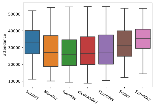
Boxplot of attendance by day of the week where weekend values are higher than weekday values
We can see here that attendance on Friday, Saturday, and Sunday is on average higher than the other days of the week. Therefore it may be beneficial to re-code this feature to eitherWeekendorWeekday.
Scaling
For quantitative features, it is important to think about how each feature is scaled. Some features will be on vastly different scales than others just based on the nature of what the feature is measuring. For example, let’s look attemperatureandtotal_runsusing the.describe()method:
bb.describe()
Copy to clipboardbb.describe()attendance temperature total_runs
count 2457.000000 2457.000000 2457.000000
mean 30380.462352 73.834959 8.949187
std 9874.626652 10.567219 4.579542
min 8766.000000 31.000000 1.000000
25% 22437.000000 67.000000 6.000000
50% 30628.000000 74.000000 8.000000
75% 38412.000000 81.000000 12.000000
max 54449.000000 101.000000 60.000000These two features are on different scales because what they are measuring are different (temperatureis in degrees Fahrenheit,total_runsis the number of runs scored in a game). Because of this, the ranges of values and the standard deviations for each are very different from one another. We can see here thattemperaturehas a standard deviation of about 10.57, whiletotal_runshas a standard deviation of about 4.58.
When working with features with largely differing scales, it is often a good idea tostandardizethe features so that they all have a mean of 0 and a standard deviation of 1.
A feature without any values close to zero may also make it more difficult to estimate and interpret the intercept of a regression model. Standardizing or otherwise re-scaling the feature can fix this issue.
Missing data
When we initially inspected the data, we saw some evidence that missing data is coded in a few different ways:
For example,temperatureuses the termUnknown,skyuses bothUnknownandNaN, andtotal_runshas-to represent a missing value. The observations with missing values will either have to be removed or replaced (with an imputed value or missing data type that Python can recognize, such asnp.NaN) in order to proceed with fitting a regression model.
Outliers
In our EDA, it is important to check for outliers and skew in the data. One way to check for outliers is to use scatter plots:
bb.plot.scatter(x = 'total_runs',y = 'attendance')
Copy to clipboard
bb.plot.scatter(x = 'total_runs',y = 'attendance')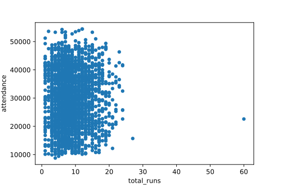
Scatter plot where the points are compressed to the left side with one extreme value on the right side
We can see here that there is one instance where the total runs in a single game is about 60, which is much larger than in the other games. Depending on the situation, we may first want to verify that this value is correct, then we can decide whether or not to remove it prior to fitting the model.
Distributions and associations
Prior to fitting a linear regression model, it can be important to inspect the distributions of quantitative features and investigate the relationships between features. We can visually inspect both of these by using a pair plot:
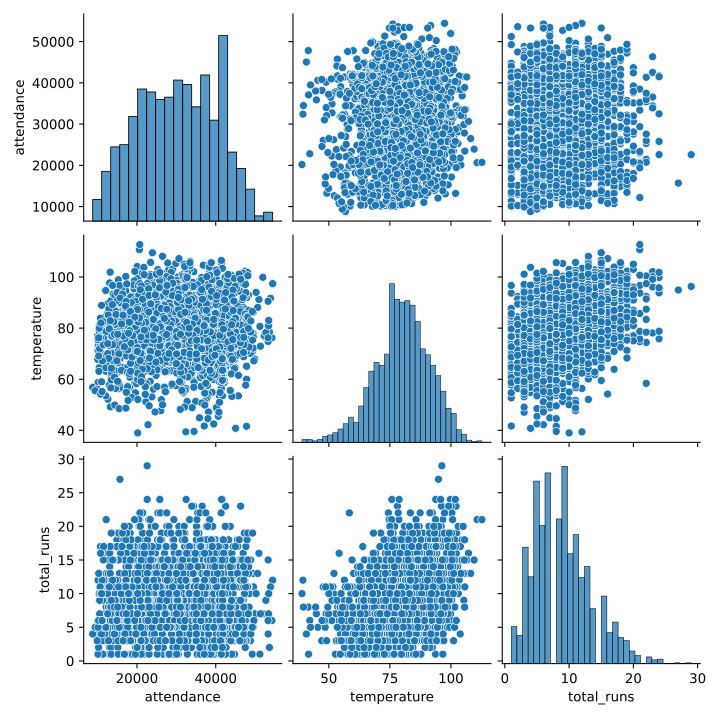
Pair plot between attendance, temperature, and total runs
Looking at the histograms along the diagonal,total_runsappears to be somewhat right-skewed. This indicates that we may want to transform this feature to make it more normally distributed.
We can explore the relationships between pairs of features by looking at the scatterplots off of the diagonal. This is useful for a few different reasons. For example, if we see non-linear associations between any of the predictors and the outcome variable, that might lead us to test out polynomial terms in our model. We can also get a sense for which features are most highly related to our outcome variable and check for collinearity. In this example, there appears to be a slight positive linear association between temperature and the total number of runs. We can further investigate this using a heat map of the correlation matrix:
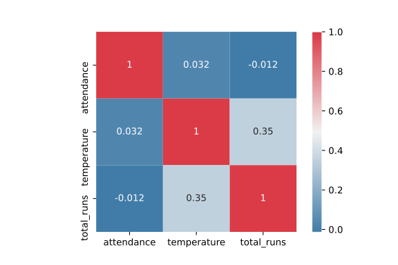
Map of the correlation between temperature, total number of runs, and attendance where stronger correlation is more darkly colored
There is a correlation of 0.35 between temperature and the total number of runs. This is not large enough to cause concern; however, if two or more predictors are highly correlated, we may consider leaving only one in our analysis. On the other hand, features that are highly correlated with our outcome variable are especially important to include in the model.
Conclusion
Let’s review the ways we were able to explore this data set in preparation for a regression model:
- We previewed the first few rows of the data set using the.head()method.
- We checked the data type of each variable in the data set using.dtypesand corrected variables with incorrect data types.
- We investigated our categorical data to inform categorical encoding.
- We investigated the scale of our quantitative variables and considered whether standardizing/scaling might be appropriate.
- We investigated missing data.
- We checked for outliers.
- We inspected the distributions of our quantitative variables.
- We looked at the relationships between pairs of features using both scatter plots and box plots.
By going through these steps, we are more prepared to make decisions about feature selection/engineering and have learned valuable information about how to build a more accurate predictive model.
'The Codecademy Team, composed of experienced educators and tech experts, is dedicated to making tech skills accessible to all. We empower learners worldwide with expert-reviewed content that develops and enhances the technical skills needed to advance and succeed in their careers.'
Complete Payment to Unlock Full Guide & Source Code
You are viewing the 30% preview. Join TopCourseAI Pro to unlock the remaining 70% of this article, unblur all code snippets, and gain full access to all 412 technical projects and guides.
Ready to access the complete step-by-step tutorial?
Gain full unhindered access to all 412 technical projects and guides, unblur all source code snippets, and download runnable scripts.
Related Blueprints & Guides
View all 166 →Creating a Word Cloud With Python
In Data Visualization,word cloudsare used to display textual data in a specific shape. The more frequent a word is in a chunk of text, the larger it will appear in the word cloud. This can provide interesting insights in...
Data visualizationData Visualizations for Messy Data
Data visualization tutorials generally use pre-processed data. But what about datasets in the wild? What do we do about missing data? Or outliers that largely skew visualizations? What do we do when there are too many ob...
Data visualizationExploratory Data Analysis with Data Visualization
Data visualization is an important component of Exploratory Data Analysis (EDA) because it allows a data analyst to “look at” their data and get to know the variables and relationships between them. In order to choose an...
Ready to build production-grade AI systems?
Enjoyed this guide? Continue exploring our library of 166+ production blueprints, multi-agent swarms, and autonomous agent systems with 100% unblurred, executable source code.