[0 1 2 3]

Use indices to get the corresponding column names of selected features:

num_cols = list(X_num.columns[selector.get_support(indices=True)])
print(num_cols)
Copy to clipboard

num_cols = list(X_num.columns[selector.get_support(indices=True)])
print(num_cols)

['hours_study', 'hours_TV', 'hours_sleep', 'height_cm']

SubsetX_numto retain only selected features:

X_num = X_num[num_cols]
print(X_num)
Copy to clipboard

X_num = X_num[num_cols]
print(X_num)

Finally, to obtain our entire features DataFrame, including the categorical columnedu_goal, we could do:

X = X[['edu_goal'] + num_cols]
print(X)
Copy to clipboard

X = X[['edu_goal'] + num_cols]
print(X)

Pearson’s correlation

Another type of filter method involves finding thecorrelationbetween variables. In particular, thePearson’s correlation coefficientis useful for measuring the linear relationship between two numeric, continuous variables — a coefficient close to1represents a positive correlation,-1represents a negative correlation, and0represents no correlation. Like variance, Pearson’s correlation coefficient cannot be calculated for categorical variables. Although, there is a relatedpoint biserial correlation coefficientthat can be computed when one variable is dichotomous, but we won’t focus on that here.

There are 2 main ways of using correlation for feature selection — to detect correlation between features and to detect correlation between a feature and the target variable.

Correlation between features

When two features are highly correlated with one another, then keeping just one to be used in the model will be enough because otherwise they provide duplicate information. The second variable would only be redundant and serve to contribute unnecessary noise.

To determine which variables are correlated with one another, we can use the.corr()method frompandasto find the correlation coefficient between each pair of numeric features in a DataFrame. By default,.corr()computes the Pearson’s correlation coefficient, but alternative methods can be specified using themethodparameter. We can visualize the resulting correlation matrix using a heatmap:

import matplotlib.pyplot as pltimport seaborn as sns
corr_matrix = X_num.corr(method='pearson')  # 'pearson' is default
sns.heatmap(corr_matrix, annot=True, cmap='RdBu_r')plt.show()
Copy to clipboard

import matplotlib.pyplot as pltimport seaborn as sns
corr_matrix = X_num.corr(method='pearson')  # 'pearson' is default
sns.heatmap(corr_matrix, annot=True, cmap='RdBu_r')plt.show()

Output:

Heatmap of corr features

Let’s define high correlation as having a coefficient of greater than0.7or less than-0.7. We canloop through the correlation matrix to identify the highly correlated variables:

# Loop over bottom diagonal of correlation matrixfor i in range(len(corr_matrix.columns)):    for j in range(i):
        # Print variables with high correlation        if abs(corr_matrix.iloc[i, j]) > 0.7:            print(corr_matrix.columns[i], corr_matrix.columns[j], corr_matrix.iloc[i, j])
Copy to clipboard

# Loop over bottom diagonal of correlation matrixfor i in range(len(corr_matrix.columns)):    for j in range(i):
        # Print variables with high correlation        if abs(corr_matrix.iloc[i, j]) > 0.7:            print(corr_matrix.columns[i], corr_matrix.columns[j], corr_matrix.iloc[i, j])

The output to our code is:

hours_TV hours_study -0.780763315142435

As seen,hours_TVappears to be highly negatively correlated withhours_study— a student who watches a lot of TV tends to spend fewer hours studying, and vice versa. Because they provide redundant information, we can choose to remove one of those variables. To decide which one, we can look at their correlation with the target variable, then remove the one that is less associated with the target. This is explored in the next section.

Correlation between feature and target

As mentioned, the second way correlation can be used is to determine if there is a relationship between a feature and the target variable. In the case of Pearson’s correlation, this is especially useful if we intend to fit a linear model, which assumes a linear relationship between the target and predictor variables. If a feature is not very correlated with the target variable, such as having a coefficient of between-0.3and0.3, then it may not be very predictive and can potentially be filtered out.

We can use the same.corr()method seen previously to obtain the correlation between the target variable and the rest of the features. First, we’ll need to create a new DataFrame containing the numeric features with theexam_scorecolumn:

X_y = X_num.copy()X_y['exam_score'] = y
print(X_y)
Copy to clipboard

X_y = X_num.copy()X_y['exam_score'] = y
print(X_y)

Then, we can generate the correlation matrix and isolate the column corresponding to the target variable to see how strongly each feature is correlated with it:

corr_matrix = X_y.corr()
# Isolate the column corresponding to `exam_score`corr_target = corr_matrix[['exam_score']].drop(labels=['exam_score'])
sns.heatmap(corr_target, annot=True, fmt='.3', cmap='RdBu_r')plt.show()
Copy to clipboard

corr_matrix = X_y.corr()
# Isolate the column corresponding to `exam_score`corr_target = corr_matrix[['exam_score']].drop(labels=['exam_score'])
sns.heatmap(corr_target, annot=True, fmt='.3', cmap='RdBu_r')plt.show()

Output:

Heatmap corr features target

As seen,hours_studyis positively correlated withexam_scoreandhours_TVis negatively correlated with it. It makes sense thathours_studyandhours_TVwould be negatively correlated with each other as we saw earlier, and just one of those features would suffice for predictingexam_score. Sincehours_studyhas a stronger correlation with the target variable, let’s removehours_TVas the redundant feature:

X = X.drop(columns=['hours_TV'])
print(X)
Copy to clipboard

X = X.drop(columns=['hours_TV'])
print(X)

The other two features,hours_sleepandheight_cm, both do not seem to be correlated withexam_score, suggesting they would not be very good predictors. We could potentially remove either or both of them as being uninformative. But before we do, it is a good idea to use other methods to double check that the features truly are not predictive. We will do that in the next section by using mutual information to see if there are any non-linear associations between the features and target variable.

To conclude this section, we’ll briefly note an alternative approach for assessing the correlation between variables. Instead of generating the full correlation matrix, we could use thef_regression()function fromscikit-learnto find the F-statistic for a model with each predictor on its own. The F-statistic will be larger (and p-value will be smaller) for predictors that are more highly correlated with the target variable, thus it will perform the same filtering:

from sklearn.feature_selection import f_regression
print(f_regression(X_num, y))
Copy to clipboard

from sklearn.feature_selection import f_regression
print(f_regression(X_num, y))

(array([3.61362007e+01, 3.44537037e+01, 0.00000000e+00, 1.70259066e-03]),
 array([3.19334945e-04, 3.74322763e-04, 1.00000000e+00, 9.68097878e-01]))

The function returns the F-statistic in the first array and the p-value in the second. As seen, the result is consistent with what we had observed in the correlation matrix — the stronger the correlation (either positive or negative) between the feature and target, the higher the corresponding F-statistic and lower the p-value. For example, amongst all the features,hours_studyhas the largest correlation coefficient (0.905), highest F-statistic (3.61e+01), and lowest p-value (3.19e-04).

Mutual information

The final filter method we’ll look at is usingmutual informationto rank and select the top features.Mutual informationis a measure of dependence between two variables and can be used to gauge how much a feature contributes to the prediction of the target variable. It is similar to Pearson’s correlation, but is not limited to detecting linear associations. This makes mutual information useful for more flexible models where a linear functional form is not assumed. Another advantage of mutual information is that it also works on discrete features or target, unlike correlation. Although, categorical variables need to be numerically encoded first.

In our example, we can encode theedu_goalcolumn using theLabelEncoderclass fromscikit-learn‘spreprocessingmodule:

from sklearn.preprocessing import LabelEncoder
le = LabelEncoder()
# Create copy of `X` for encoded versionX_enc = X.copy()X_enc['edu_goal'] = le.fit_transform(X['edu_goal'])
print(X_enc)
Copy to clipboard

from sklearn.preprocessing import LabelEncoder
le = LabelEncoder()
# Create copy of `X` for encoded versionX_enc = X.copy()X_enc['edu_goal'] = le.fit_transform(X['edu_goal'])
print(X_enc)

Now, we can compute the mutual information between each feature andexam_scoreusingmutual_info_regression(). This function is used because our target variable is continuous, but if we had a discrete target variable, we would usemutual_info_classif(). We specify therandom_statein the function in order obtain reproducible results:

from sklearn.feature_selection import mutual_info_regression
print(mutual_info_regression(X_enc, y, random_state=68))
Copy to clipboard

from sklearn.feature_selection import mutual_info_regression
print(mutual_info_regression(X_enc, y, random_state=68))

[0.50396825 0.40896825 0.06896825 0.        ]

The estimated mutual information between each feature and the target is returned in a numpy array, where each value is a non-negative number — the higher the value, the more predictive power is assumed.

However, we are missing one more important piece here. Earlier, even though we encodededu_goalto be numeric, that does not mean it should be treated as a continuous variable. In other words, the values ofedu_goalare still discrete and should be interpreted as such. If we plotedu_goalagainstexam_scoreon a graph, we can clearly see the steps between the values ofedu_goal:

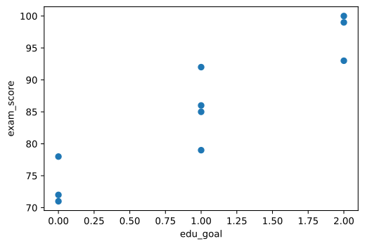
Scatterplot of education goals against exam scores

In order to properly calculate the mutual information, we need to tellmutual_info_regression()which features are discrete by providing their index positions using thediscrete_featuresparameter:

print(mutual_info_regression(X_enc, y, discrete_features=[0], random_state=68))
Copy to clipboard

print(mutual_info_regression(X_enc, y, discrete_features=[0], random_state=68))

[0.75563492 0.38896825 0.18563492 0.        ]

Compared to the earlier results, we now get greater mutual information betweenedu_goaland the target variable once it is correctly interpreted as a discrete feature.

From the results, we can also see that there is0mutual information betweenheight_cmandexam_score, suggesting that these variables are largely independent. This is consistent with what we saw earlier with Pearson’s correlation, where the correlation coefficient between them is very close to0as well.

What is interesting to note is that the mutual information betweenhours_sleepandexam_scoreis a positive value, even though their Pearson’s correlation coefficient is0. The answer becomes more clear when we plot the relationship betweenhours_sleepandexam_score:

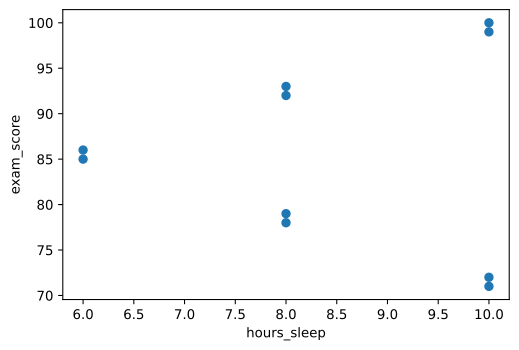
Scatterplot of hours slept against exam scores

As seen, there do seem to be some association between the variables, only it is not a linear one, which is why it was detected using mutual information but not Pearson’s correlation coefficient.

Finally, let’s look at using theSelectKBestclass fromscikit-learnto help pick out the topkfeatures with the highest ranked scores. In our case, we are looking to select features that share the most mutual information with the target variable. When we instantiateSelectKBest, we’ll specify which scoring function to use and how many top features to select. Here, our scoring function ismutual_info_regression(), but because we want to specify additional arguments besides theXandyinputs, we’ll need the help of thepartial()function from Python’s built-infunctoolsmodule. Then, the.fit_transform()method will return the filtered features as a numpy array:

from sklearn.feature_selection import SelectKBestfrom functools import partial
score_func = partial(mutual_info_regression, discrete_features=[0], random_state=68)
# Select top 3 features with the most mutual informationselection = SelectKBest(score_func=score_func, k=3)
print(selection.fit_transform(X_enc, y))
Copy to clipboard

from sklearn.feature_selection import SelectKBestfrom functools import partial
score_func = partial(mutual_info_regression, discrete_features=[0], random_state=68)
# Select top 3 features with the most mutual informationselection = SelectKBest(score_func=score_func, k=3)
print(selection.fit_transform(X_enc, y))

[[ 0  1 10]
 [ 0  2 10]
 [ 0  3  8]
 [ 1  3  8]
 [ 1  3  6]
 [ 1  4  6]
 [ 1  3  8]
 [ 2  4  8]
 [ 2  5 10]
 [ 2  5 10]]

As seen above, we selected the top 3 features based on mutual information, thus droppingheight_cm. LikeVarianceThreshold,SelectKBestalso offers the.get_support()method that returns the indices of the selected features, so we could subset our original features DataFrame:

X = X[X.columns[selection.get_support(indices=True)]]
print(X)
Copy to clipboard

X = X[X.columns[selection.get_support(indices=True)]]
print(X)

Conclusion

In our example dataset, we started out with 6 features for predicting theexam_scoreof students. Using various filter methods, we narrowed down that set to just the top most relevant and informative ones. First, we eliminatedgrade_levelbecause it has zero variance and would contribute nothing to the model. Then, we droppedhours_TVsince it is highly correlated withhours_studyand is therefore redundant. Lastly, we filtered outheight_cmbased on mutual information, which suggested that it does not have any meaningful association with the target variable, linear or otherwise, and would not have been very predictive.

Phew! That was a lot we were able to accomplish using filter methods. Being the most simple type of feature selection method, they sure do not lack power nor potential. It is certainly worth considering how you might want to incorporate filter methods into your next machine learning project.

'The Codecademy Team, composed of experienced educators and tech experts, is dedicated to making tech skills accessible to all. We empower learners worldwide with expert-reviewed content that develops and enhances the technical skills needed to advance and succeed in their careers.'