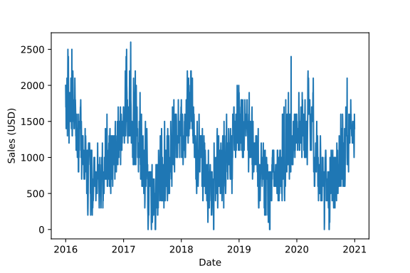
Line plot showing year on the x-axis and sales in USD on the y-axis

Notice how we can see the trend of the data over time. Looking at the chart, it seems that:

• Sales are seasonal, peaking at the beginning and end of each year, and slowing down in the middle of each year.
• Sales don’t seem to show signs of growth over time. This appears to be a stagnant business.

Box plot

When working with time series data, box plots can be useful to see the distribution of values grouped by time interval.

For example, let’s create a box plot for each year of sales and put them side-to-side for comparison:

# extract year from date columnsales_data["year"] = sales_data["date"].dt.year
# box plot grouped by yearsns.boxplot(data=sales_data, x="year", y="sales")plt.show()
Copy to clipboard

# extract year from date columnsales_data["year"] = sales_data["date"].dt.year
# box plot grouped by yearsns.boxplot(data=sales_data, x="year", y="sales")plt.show()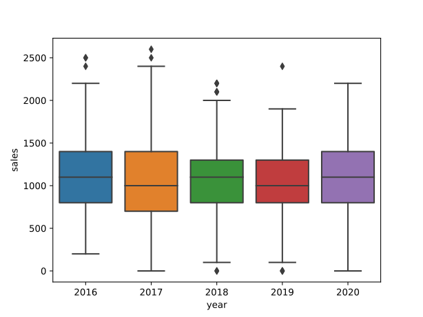

Side-by-side box plots for each year of sales showing that median sales are flat over time

For each year of the sales data, we can easily see useful information such as median sales, the highest and lowest sales, the interquartile range of our data, and any outliers.

Median sales for each year (represented by the horizontal line in each box) are quite stable, suggesting that sales are not growing over time.

Heatmap

We can also use a heatmap to compare observations between time intervals in time series data.

For example, let’s create a density heatmap with year on the y-axis and month on the x-axis. This can be done by invoking theheatmap()function of thesnsSeaborn object:

# calculate total sales for each monthsales = sales_data.groupby(["year", "month"]).sum()
# re-format the data for the heat-mapsales_month_year = sales.reset_index().pivot(index="year", columns="month", values="sales")
# create heatmapsns.heatmap(sales_month_year, cbar_kws={"label": "Total Sales"})plt.title("Sales Over Time")plt.xlabel("Month")plt.ylabel("Year")plt.show()
Copy to clipboard

# calculate total sales for each monthsales = sales_data.groupby(["year", "month"]).sum()
# re-format the data for the heat-mapsales_month_year = sales.reset_index().pivot(index="year", columns="month", values="sales")
# create heatmapsns.heatmap(sales_month_year, cbar_kws={"label": "Total Sales"})plt.title("Sales Over Time")plt.xlabel("Month")plt.ylabel("Year")plt.show()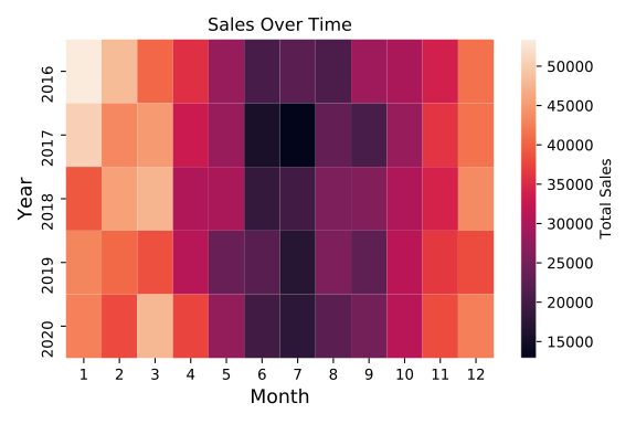

heat map of total sales with month on the x-axis and year on the y-axis

Recall that in a heatmap, as the color gets brighter and moves from dark purple to yellow, the total sales in the corresponding cell is higher.

Here, we see once again that the sales are pretty consistent year after year and also exhibit seasonality.

Lag scatter plot

We can use alag scatter plotto explore the relationship between an observation and a lag of that observation.

In a time series, alagis a previous observation:

• The observation at a previous time step (the smallest time interval for which we have distinct measurements) is called lag 1.
• The observation at two times ago is called lag 2, etc.

In the sales dataset, we have a different sales value for each day. Therefore, the lag 1 value for any particular day is equal to the sales on the previous day. The lag 2 value is the sales two days ago, etc.

Theplottingmodule of thepandaslibrary has a built-inlag_plotfunction that plots the observation at time t on the x-axis and the lag 1 observation (t+1) on the y-axis:

# import lag_plot functionfrom pandas.plotting import lag_plot
# lag scatter plotlag_plot(sales_data)plt.show()
Copy to clipboard

# import lag_plot functionfrom pandas.plotting import lag_plot
# lag scatter plotlag_plot(sales_data)plt.show()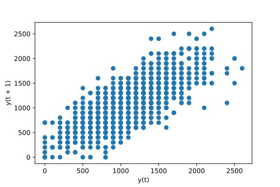

Example of a lag scatter plot using sales data

How can we interpret a lag scatter plot?

• If the points move from the bottom left to the top right, this indicates a positive correlation between observations and their lag 1 values. For example, high sales on one day are associated with high sales on the previous day.
• If the points move from the top left to the bottom right, this indicates a negative correlation between observations and their lag 1 values. For example, high sales on one day are associated with low sales on the previous day and vice versa.
• If there is no identifiable structure in the lag plot, this indicates the data is random, and there is no association between values at consecutive time points. For example, sales on one day tell you no information about expected sales on the following day.

Exploring the relationship between an observation and a lag of that observation is useful for helping us determine whether a dataset is random.

Since the points in the sales data move along a diagonal line from the bottom left to the top right, this indicates that our data is not random and there is a positive correlation between observations and their lag 1 values.

Autocorrelation plot

Anautocorrelation plotis used to show whether the elements of a time series are positively correlated, negatively correlated, or independent of each other.

This can be plotted with theautocorrelation_plot()function of thepandas.plottingmodule:

# import autocorrelation functionfrom pandas.plotting import autocorrelation_plot
# autocorrelation plotautocorrelation_plot(sales_data)plt.show()
Copy to clipboard

# import autocorrelation functionfrom pandas.plotting import autocorrelation_plot
# autocorrelation plotautocorrelation_plot(sales_data)plt.show()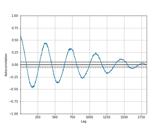

Autocorrelation plot for sales data with lag on the x-axis and the value of the autocorrelation on the y-axis

In the autocorrelation plot above, lag is on the x-axis and the value of the autocorrelation, which ranges from -1 to 1, is on the y-axis. A value near 0 indicates a weak correlation while values closer to -1 and 1 indicate a strong correlation.

Notice how the autocorrelation plot for the sales data forms waves, oscillating between strong negative and positive correlation. These waves suggest that our dataset exhibits seasonality.

Also, notice how the autocorrelation decreases over time. This indicates that sales tend to be similar on consecutive days, but sales from three years ago are less associated with today’s sales than sales from one year ago.

Review

In this article, you got a brief introduction to exploring and visualizing time series data using:

As a Data Scientist or Analyst, you will often work with data that changes over time. Moving forward, you are now better equipped to explore and visualize data with a time component.

'The Codecademy Team, composed of experienced educators and tech experts, is dedicated to making tech skills accessible to all. We empower learners worldwide with expert-reviewed content that develops and enhances the technical skills needed to advance and succeed in their careers.'