
Introduction to Data Wrangling and Tidying
Introduction to Data Wrangling and Tidying
Frequently when we work with data, we encounter unstructured and/ormessy data. Messy data can take a variety of forms. This could mean any of the following:
- The columns are mislabeled or do not have variable names.
- The dataset contains nonsensical data.
- Variables are stored in both the columns and rows.
While the data may be messy, it is still extremely informative. We need to clean, transform, and sometimes manipulate the data structure to gain any insights. This process is often calleddata wranglingordata munging.
At the final stages of the data wrangling process, we will have a dataset that we can easily use for modeling purposes or for visualization purposes. This is atidydataset where each column is a variable and each row is an observation.
Data Wrangling
Let’s look at a subset of restaurant inspections from theNew York City Department of Health and Mental Hygiene(NYC DOHMH) to work through some data wrangling processes. The data includes seven different columns with information about a restaurant’s location and health inspection. Here is a description of the dataset’s variables.
Pos.    Var. Name                 Var. Description
-----   --------------------      --------------------------------------
0       DBA                       Restaurant name
1       BORO                      Borough
2       CUISINE DESCRIPTION       Type of cuisine
3       GRADE                     Letter grade
4       LATITUDE                  Latitude coordinates of restaurant
5       LONGITUDE                 Longitude coordinates of restaurant
6       URL                       URL link to restaurant's website
Let’s use theread_csv()function inpandasto load our dataset as a pandas dataframe and take a look at the first 10 rows out of the 27 total.
import pandas as pdrestaurants = pd.read_csv("DOHMH_restaurant_inspections.csv")
# the .head(10) function will show us the first 10 rows in our datasetprint(restaurants.head(10))
Copy to clipboard
import pandas as pdrestaurants = pd.read_csv("DOHMH_restaurant_inspections.csv")
# the .head(10) function will show us the first 10 rows in our datasetprint(restaurants.head(10))Output:
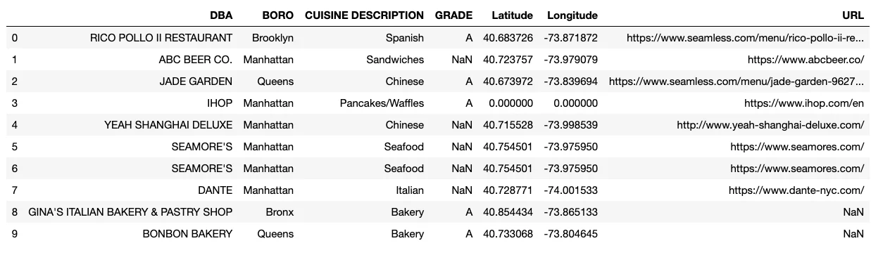
data_wrangling_data1_restaurants
The.shapemethod in pandas identifies the number of rows and columns in our dataset as (rows, columns):
restaurants.shape
Copy to clipboardrestaurants.shapeOutput:
(27, 7)When we look closely at the table, we see some missing data. In bothGRADEandURLcolumns, we have missing values marked as NaNs. In theLatitudeandLongitudecolumns, we have a missing set of coordinates marked as (0.000, 0.000) for IHOP. (0.000, 0.000) is the label for missing coordinates because no restaurants in New York City are at the equator. Other common indicators used for missing values are values that are NA and -.
Preliminary data cleaning
There are also duplicate rows for the restaurant labeled Seamore’s. To remove any duplicate rows, we can use thedrop_duplicates()function
# the .drop_duplicates() function removes duplicate rowsrestaurants = restaurants.drop_duplicates()
# the .head(10) function will show us the first 10 rows in our datasetprint(restaurants.head(10))
Copy to clipboard
# the .drop_duplicates() function removes duplicate rowsrestaurants = restaurants.drop_duplicates()
# the .head(10) function will show us the first 10 rows in our datasetprint(restaurants.head(10))Output:
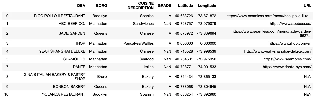
data_wrangling_restaurants_drop_duplicate
The.shapemethod again:
restaurants.shape
Copy to clipboardrestaurants.shape(25, 7)After dropping duplicate rows, we are left with 25 rows and can now see “YOLANDA RESTAURANT” at the bottom when looking at our dataset’s first 10 rows.
If we look at the first four columns of our data:DBA,BORO,CUISINE DESCRIPTION, andGRADE. These column names are all capitalized, while the columns following it use both uppercase and lowercase. To have some consistency across column names, we will iterate over the column names of our dataset and convert them all to lowercase using themap()andlower()functions. We also need to make sure to include thestrfunction to identify that we are working with strings.
# map() applies the str.lower() function to each of the columns in our dataset to convert the column names to all lowercaserestaurants.columns = map(str.lower, restaurants.columns)
# the .head(10) function will show us the first 10 rows in our datasetprint(restaurants.head(10))
Copy to clipboard
# map() applies the str.lower() function to each of the columns in our dataset to convert the column names to all lowercaserestaurants.columns = map(str.lower, restaurants.columns)
# the .head(10) function will show us the first 10 rows in our datasetprint(restaurants.head(10))Output:
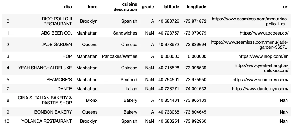
data_wrangling_restaurants_lower
You may have noticed that the first column of the dataset is calledDBA, but we know it is a column with restaurant names. We can use therename()function and a dictionary to relabel our columns. While we are renaming our columns, we might also want to shorten thecuisine descriptioncolumn to justcuisine.
# axis=1` refers to the columns, `axis=0` would refer to the rows# In the dictionary the key refers to the original column name and the value refers to the new column name {'oldname1': 'newname1', 'oldname2': 'newname2'}restaurants = restaurants.rename({'dba': 'name', 'cuisine description': 'cuisine'}, axis=1)

# the .head(10) function will show us the first 10 rows in our datasetprint(restaurants.head(10))
Copy to clipboard
# axis=1` refers to the columns, `axis=0` would refer to the rows# In the dictionary the key refers to the original column name and the value refers to the new column name {'oldname1': 'newname1', 'oldname2': 'newname2'}restaurants = restaurants.rename({'dba': 'name', 'cuisine description': 'cuisine'}, axis=1)
# the .head(10) function will show us the first 10 rows in our datasetprint(restaurants.head(10))Output:
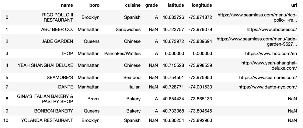
data_wrangling_restaurants_cols_named
Data Types
Great! Now we have a dataset that is cleaner and much easier to read!. Let’s take a look at each column’s data types by appending.dtypesto our pandas dataframe.
restaurants.dtypes
Copy to clipboardrestaurants.dtypesname object
boro object
cuisine object
grade object
latitude float64
longitude float64
url object
dtype: objectWe have two types of variables: object and float64.objectcan consist of both strings or mixed types (both numeric and non-numeric), andfloat64are numbers with afloating point(ie. numbers with decimals). There are other data types such asint64(integer numbers),bool(True/False values), anddatetime64(date and/or time values).
Since we have both continuous (float64) and categorical (object) variables in our data, it might be informative to look at the number of unique values in each column using thenunique()function.
# .nunique() counts the number of unique values in each column restaurants.nunique()
Copy to clipboard
# .nunique() counts the number of unique values in each column restaurants.nunique()name 25
boro 4
cuisine 15
grade 1
latitude 24
longitude 24
url 16We see that our data consists of 4 boroughs in New York and 15 cuisine types. We know that we also have missing data inurlfrom our initial inspection of the data, so the unique number of values inurlmight not be super informative. Additionally, we have corrected for duplicate restaurants, so the restaurant name, latitude, longitude, and url should be unique to each restaurant (unless, of course, there are some restaurant chains at different locations).
Missing Data
From our initial inspection of the data, we know we have missing data ingrade,url,latitude, andlongitude. Let’s take a look at how the data is missing, also referred to asmissingness. To do this we can useisna()to identify if the value is missing. This will give us a boolean and indicate if the observation in that column is missing (True) or not (False). We will also usesum()to count the number of missing values, whereisna()returns True.
# counts the number of missing values in each column restaurants.isna().sum()
Copy to clipboard
# counts the number of missing values in each column restaurants.isna().sum()name 0
boro 0
cuisine 0
grade 15
latitude 0
longitude 0
url 9We see that there are missing values in the grade and url columns, but no missing values inlatitudeandlongitude. However, coordinates at (0.000, 0.000) are not valid for any of the restaurants in our dataset, and we saw that these exist in our initial analysis. To handle this, we will replace the (0.000, 0.000) coordinates with NaN values.
We will use the.where()method from thepandaslibrary to replace the invalid coordinates. The.where()method keeps the values specified in its first argument, and replaces all other values withNaN.
# here our .where() function replaces latitude values less than 40 with NaN valuesrestaurants['latitude'] = restaurants['latitude'].where(restaurants['latitude'] > 40)
# here our .where() function replaces longitude values greater than -70 with NaN valuesrestaurants['longitude'] = restaurants['longitude'].where(restaurants['longitude'] < -70)
# .sum() counts the number of missing values in each columnrestaurants.isna().sum()
Copy to clipboard
# here our .where() function replaces latitude values less than 40 with NaN valuesrestaurants['latitude'] = restaurants['latitude'].where(restaurants['latitude'] > 40)
# here our .where() function replaces longitude values greater than -70 with NaN valuesrestaurants['longitude'] = restaurants['longitude'].where(restaurants['longitude'] < -70)
# .sum() counts the number of missing values in each columnrestaurants.isna().sum()name 0
boro 0
cuisine 0
grade 15
latitude 2
longitude 2
url 9Now we see that latitude and longitude each have two missing data points thanks to replacing the (0.000, 0.000) values with NaN values.
Let’s try to understand the missingness in theurlcolumn by counting the missing values across each borough. We will use thecrosstab()function in pandas to do this.
Thecrosstab()computes the frequency of two or more variables. To look at the missingness in theurlcolumn we can addisna()to the column to identify if there is an NaN in that column. This will return a boolean, True if there is a NaN and False if there is not. In our crosstab, we will look at all the boroughs present in our data and whether or not they have missing url links.
pd.crosstab(         # tabulates the boroughs as the index        restaurants['boro'],
        # tabulates the number of missing values in the url column as columns        restaurants['url'].isna(),
        # names the rows        rownames = ['boro'],
        # names the columns         colnames = ['url is na'])
Copy to clipboard
pd.crosstab( # tabulates the boroughs as the index restaurants['boro'],
# tabulates the number of missing values in the url column as columns restaurants['url'].isna(),
# names the rows rownames = ['boro'],
# names the columns colnames = ['url is na'])url is na False True
boro
Bronx 1 1
Brooklyn 2 4
Manhattan 11 2
Queens 2 2We see that most of the restaurants in Manhattan in our dataset have restaurant links, while most restaurants in Brooklyn do not have url links.
Removing prefixes
It might be easier to read what url links are by removing the prefixes of the websites, such as “https://www.”. We will usestr.lstrip()to remove the prefixes. Similar to when we were working with our column names, we need to make sure to include thestrfunction to identify that we are working with strings andlstripto remove parts of the string from the left side.
# .str.lstrip('https://') removes the “https://” from the left side of the stringrestaurants['url'] = restaurants['url'].str.lstrip('https://')
# .str.lstrip('www.') removes the “www.” from the left side of the stringrestaurants['url'] = restaurants['url'].str.lstrip('www.')
# the .head(10) function will show us the first 10 rows in our datasetprint(restaurants.head(10))
Copy to clipboard
# .str.lstrip('https://') removes the “https://” from the left side of the stringrestaurants['url'] = restaurants['url'].str.lstrip('https://')
# .str.lstrip('www.') removes the “www.” from the left side of the stringrestaurants['url'] = restaurants['url'].str.lstrip('www.')
# the .head(10) function will show us the first 10 rows in our datasetprint(restaurants.head(10))Output:

data_wrangling_restaurants_url_cleaned
Amazing! Our dataset is now much easier to read and use. We have identifiable columns and variables that are easy to work with thanks to our data wrangling process. We also corrected illogical data values and made the strings a little easier to read.
In this example, we worked with data that was rathertidy, in the sense that each row was an observation (a restaurant) and each column was a variable. However, what if our dataset was not tidy? What if our columns and rows needed reorganization?
Tidy Data
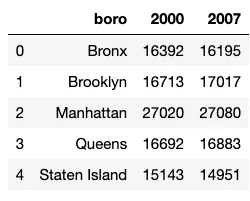
Let’s take a look at a dataset that has information about the average annual wage for restaurant workers across New York City boroughs and New York City as a whole from the years 2000 and 2007. The data is from theNew York State Department of Labor, Quarterly Census of Employment and Wages,and only contains six total rows.
annual_wage = pd.read_csv("annual_wage_restaurant_boro.csv")print(annual_wage)
Copy to clipboard
annual_wage = pd.read_csv("annual_wage_restaurant_boro.csv")print(annual_wage)Output:
data_wrangling_annual_wage_data
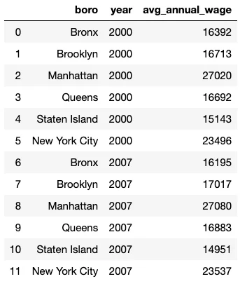
There are three variables in this dataset:borough,year, andaverage annual income. However, we have values (2000 and 2007) in the column headers rather than variable names (yearandaverage annual income). This is not ideal to work with, so let’s fix it! We will use themelt()function in pandas to turn the current values (2000 and 2007) in the column headers into row values and addyearandavg_annual_wageas our column labels.
annual_wage=annual_wage.melt(
      # which column to use as identifier variables      id_vars=["boro"],             # column name to use for “variable” names/column headers (ie. 2000 and 2007)       var_name=["year"],
      # column name for the values originally in the columns 2000 and 2007      value_name="avg_annual_wage")
print(annual_wage)
Copy to clipboard
annual_wage=annual_wage.melt(
# which column to use as identifier variables id_vars=["boro"], # column name to use for “variable” names/column headers (ie. 2000 and 2007) var_name=["year"],
# column name for the values originally in the columns 2000 and 2007 value_name="avg_annual_wage")
print(annual_wage)Output:
data_wrangling_annual_wage_data_long
Now we have a tidy dataset where each column is a variable (borough, year, or average annual wage), and each row is an observation! This dataset will be much easier to work with moving forward!
You now have the tools to continue to gather more information about New York City restaurants to answer questions you are interested in exploring. For example, we could explore what variables are most predictive of receiving a passing health score. We would need to gather some more data and go through the data wrangling process to end up with tidy data that is ready for analysis. Happy coding!
'The Codecademy Team, composed of experienced educators and tech experts, is dedicated to making tech skills accessible to all. We empower learners worldwide with expert-reviewed content that develops and enhances the technical skills needed to advance and succeed in their careers.'
Complete Payment to Unlock Full Guide & Source Code
You are viewing the 30% preview. Join TopCourseAI Pro to unlock the remaining 70% of this article, unblur all code snippets, and gain full access to all 412 technical projects and guides.
Ready to access the complete step-by-step tutorial?
Gain full unhindered access to all 412 technical projects and guides, unblur all source code snippets, and download runnable scripts.
Related Blueprints & Guides
View all 166 →Accessibility on the Platform
Codecademy is committed to providing a high-quality learning experience for all learners. That includes accommodating different usage forms such as auditory, motor, or visual restrictions, limited hardware, or other acce...
Web developmentAffordances, Signifiers, and Clickability
For users on the web, the mouse click is perhaps the most fundamental human-computer interaction. The webbecamethe web partially through the power ofhypertext, or text in one document that links to other documents or res...
Web developmentAuthentication and OAuth
Authenticationis the process used by applications to determine and confirm identities of users. It ensures that the correct content is shown to users. More importantly, it ensures that incorrect content is secured and u...
Ready to build production-grade AI systems?
Enjoyed this guide? Continue exploring our library of 166+ production blueprints, multi-agent swarms, and autonomous agent systems with 100% unblurred, executable source code.