In this representation, thebeta values(B_0andB_1) represent the regression coefficients. In high school, we are often taught that a line can be formally represented as follows:

Y=m∗x+bY = m*x + b
Y=m∗x+b

Our simple regression model follows the same formula. Except, in our case them, orslopevalue, is represented by B_1 and theb, or intercept value, represented byB_0. Regression analysis finds the best fit values for B_0 and B_1 and allows for us to describe the relationship between two variables using the resulting equation of the best fit line.

So how does a regression model find these beta values? In most cases, the best fit line is agreed to be the most that minimizes theresidual error. A model will never perfectly fit the data, so there will always be some error, or difference between the actual observed data value and the value predicted by a model. This difference is commonly referred to as aresidual, and is formally represented as follows:

Errori=yi−y^iError_i = y_i - \hat{y}_i
Errori​=yi​−y^​i​

A very naive approach model for data prediction would just predict that the value of a new data point will equal the average of all observed data. This model would look like the example below, where the model’s predictions are represented by a red line:

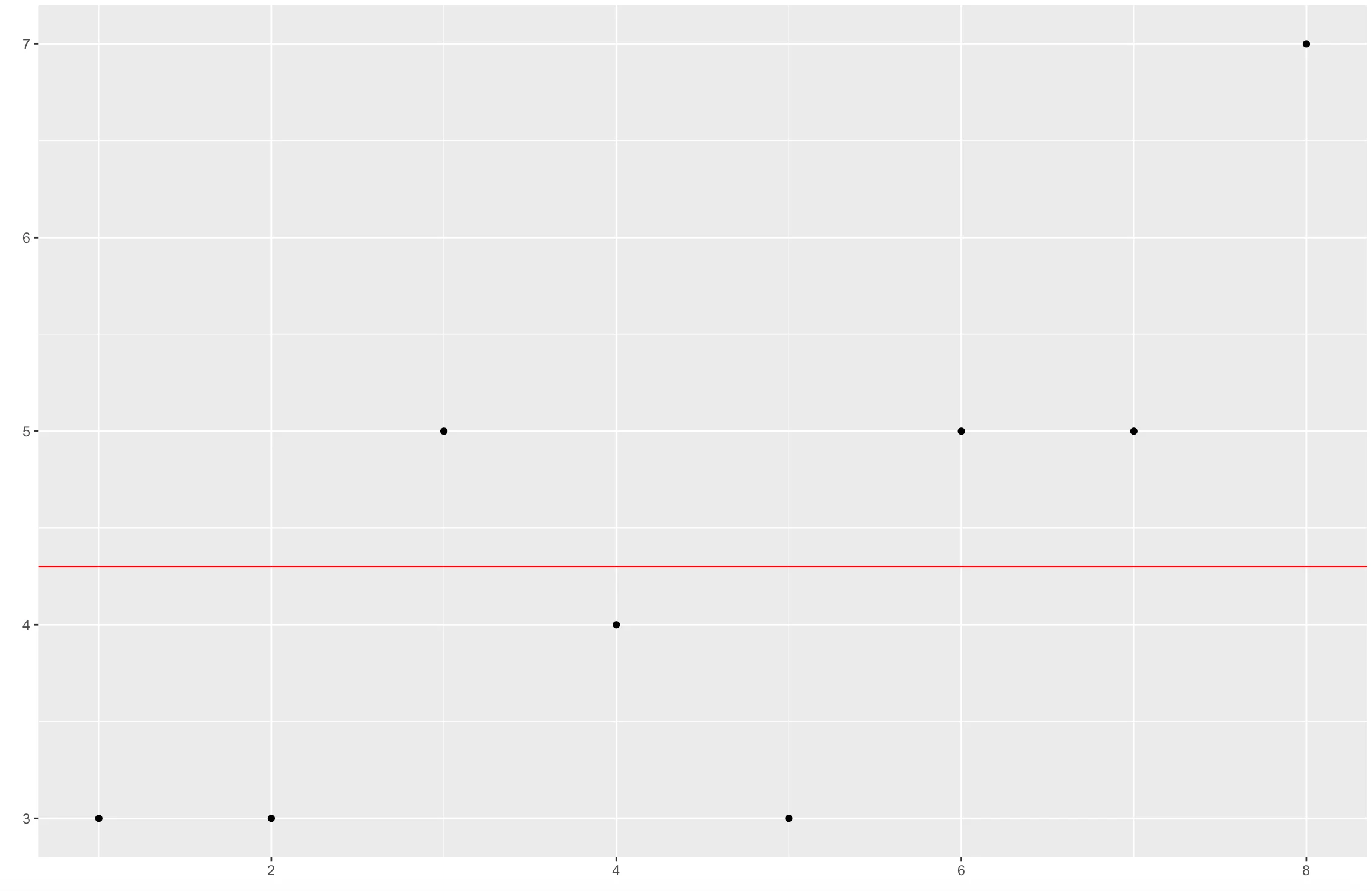
This model doesn’t seem like it fits our data very well. If we drew a line from our observed data points to the prediction line, as shown below, then added up the absolute length of all these lines, oursum of residual errorwould be equal to 9. Any line that has a lower sum of residual error than our naive model would be considered a better fit line.

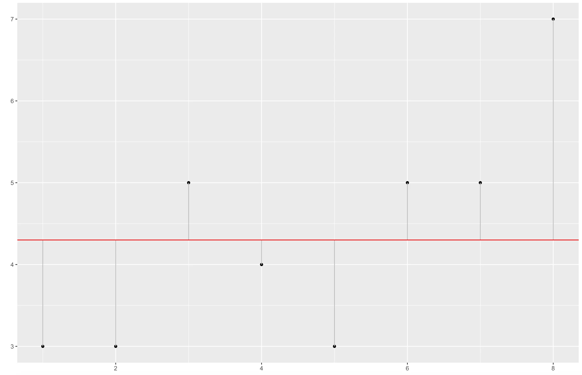
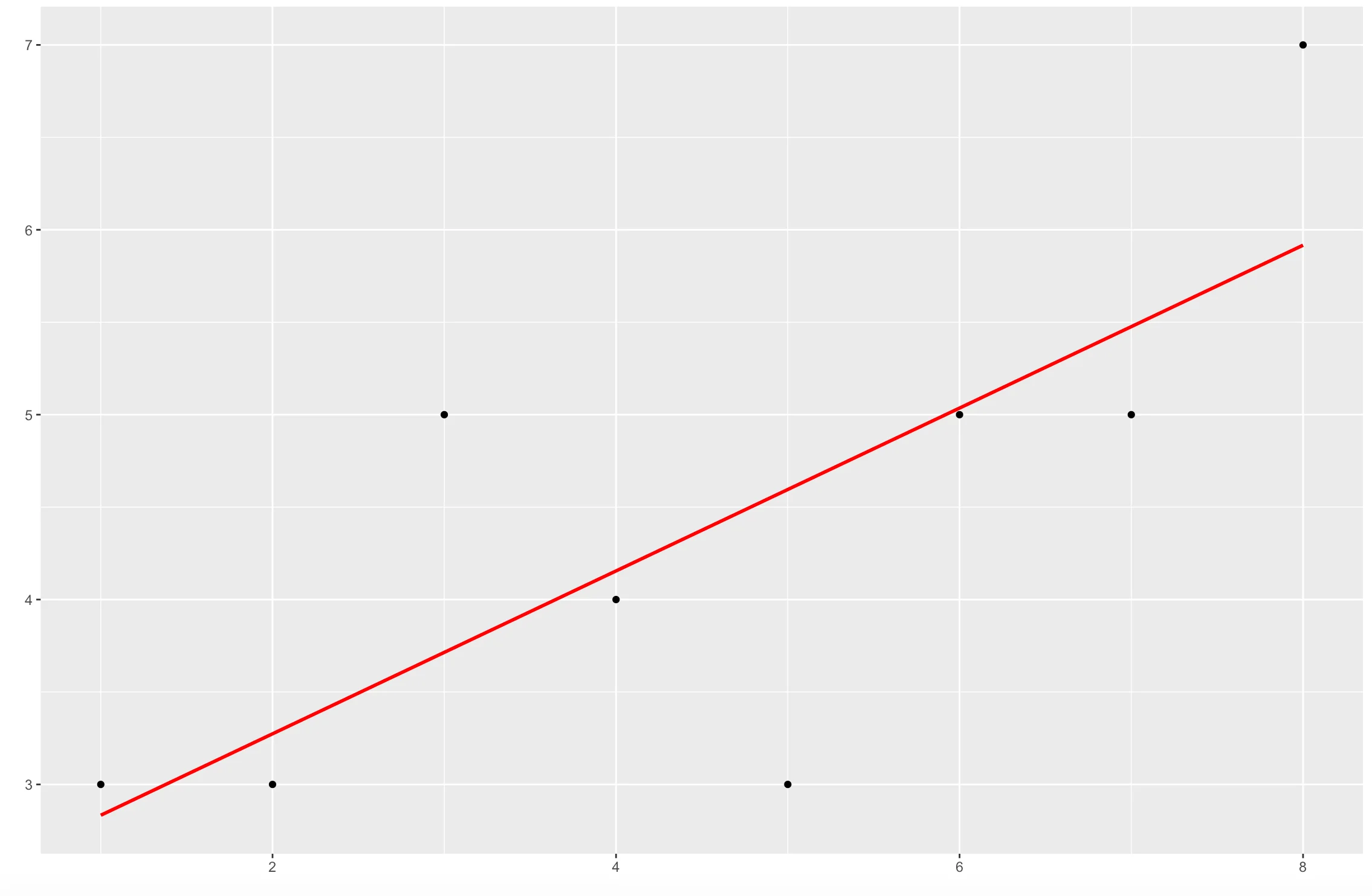
However, it is important to note that regression models use thesum ofsquarederror (SSE); in our example above, our naive model has a SSE of 13.92. We use squared error because a prediction can either be greater than or less than the actual value, producing a positive or negative error value. We avoided this issue in our calculation above by taking the absolute difference between observed and predicted values. But, If we did not square the error values or take their absolute difference, the sum of errors could decrease because of negative error values, not because a model fits the data best. While absolute difference solves this issue, it is far more common to fit a model based on squared errors. The square function adds a greater penalty to predicted values that are very incorrect, as squaring larger values results in a respectively larger result than squaring small values, this helps bias the model fitting calculation towards a line that produces accurate predictions forallvalues in a dataset, rather than a handful of most common observations. The example below shows a line fit by selecting the beta coefficients that have minimized SSE to 5.38. Doesn’t that line look better?

Assess Model Fit

While theoretically the sum of square error gives us the best fit model given the data at hand, it doesn’t guarantee that this best model is actually a “good”, or relatively accurate, model. There are a number of statistics used to summarize model fit, but one of the most common measures isR-squared, sometimes called the coefficient of determination. R-squared quantifies theproportion of the variability in the outcome variable that can be explained by a predictor variable. More simply, it summarizes the difference between the sum of squared error for a line which is simply the average of all Y values, or outcome variables, and the sum of squared error for our proposed model. It can be formally represented as follows:

SStotal=sumi(yi−yhati)2SS_{total} = sum_i ( y_i - y^hat_i)^2
SStotal​=sumi​(yi​−yhati​)2

SSresidual=sumi(yi−f(xi))2SS_{residual} = sum_i ( y_i -  f(x_i))^2
SSresidual​=sumi​(yi​−f(xi​))2

R2=1−SSresidual/SStotalR^2 = 1- SS_{residual}/SS_{total}
R2=1−SSresidual​/SStotal​

In this case, SS_total represents the squared difference between the actual data and the average value of all Y values, and SS_residual represents the squared difference between the actual data and the values predicted by our model. We saw in our example model above that the SS_total for our model was 13.92, and the SS_residual was 5.38. The R-squared calculation is simply one minus the proportion of our total and residual sum of squares; plugging in the values from our example, we get an R-squared value of 0.61:

R2=1−5.38/13.92R^2 = 1- 5.38/13.92
R2=1−5.38/13.92

0.61=1−0.38640.61 = 1 - 0.3864
0.61=1−0.3864

This means that if predictor variable X can predict the outcome variable with consistent accuracy, then the proportion is high and the R-squared value will be close to 1. If the opposite is true, the R-squared value is closer to 0. We can provide a narrative around the R-squared value by saying that: “ [R-squared value] percent of the variation in [outcome variable] is explained (or predicted) by [predictor variable]”. In our example. 61% of the variation our Y value is explained by our X value. That’s pretty good!

This is just the beginning of regression analysis! For the past two centuries researchers have been developing innovative approaches to regression-based analysis. By building up your theoretical and technical understanding of regression models, you too can join the ranks of statisticians utilizing the most widely and consistently applied methods to better understand our world.

'The Codecademy Team, composed of experienced educators and tech experts, is dedicated to making tech skills accessible to all. We empower learners worldwide with expert-reviewed content that develops and enhances the technical skills needed to advance and succeed in their careers.'